Linear Algebra Preview

A peek under the hood

Consider the linear system of equations

\[1.5x + 0.5y = 2\]

«««< HEAD $0.2x + 1.2y = 1.4$ ======= \(0.2x + 1.2y = 1.2\)

b03dea6aa00d7330189d6f3f8b24cde6cb96ef22

If we solve this system of equations using algebraic techniques, we can trivially find that $x = 1$ and $y = 1$

Using matrices, we can also write this system as

\[\begin{bmatrix} 1.5 & 0.5\\ 0.2 & 1.2\\ \end{bmatrix} \begin{bmatrix} x\\ y\\ \end{bmatrix} = \begin{bmatrix} 2\\ 1.2\\ \end{bmatrix}\]

Transformation Visualization

Motivation: Why Matrices?

Matrix notation is visually cumbersome, and it is often difficult to understand. However, for complicated systems, it often simplifies calculations. Further, computing software such as MATLAB can help solve these systems quickly.

Consider the Lorentz Equation (Model to show Atmospheric Convection) which can be visualized as

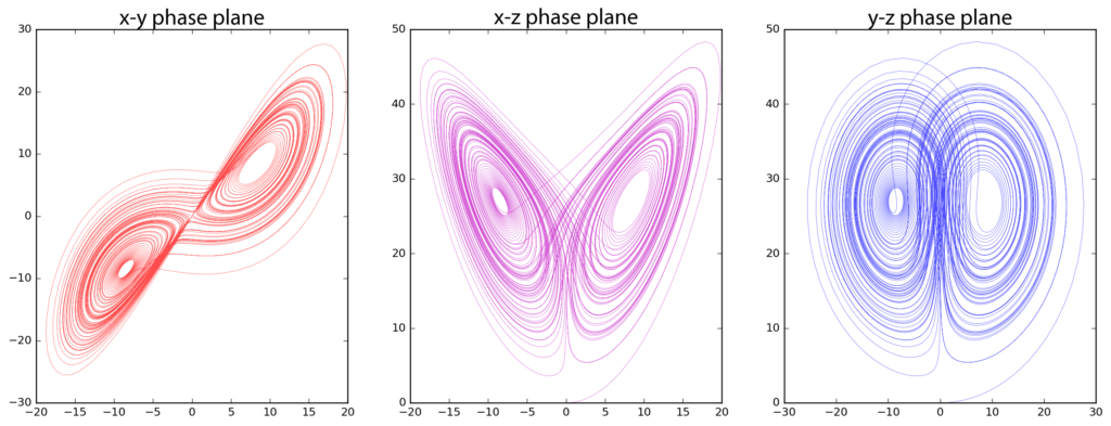
We can write this system of ODEs as

\[\begin{cases} \frac{dx}{dt} = \sigma(y - x) \\ \frac{dy}{dt} = x(\rho - z) - y \\ \frac{dz}{dt} = xy - \beta z \\ x(0) = x_0, \quad y(0) = y_0, \quad z(0) = z_0 \end{cases}\]

We can solve this system in matrix form as

\[\frac{d}{dt} \begin{pmatrix} x \\ y \\ z \end{pmatrix} = \begin{pmatrix} -\sigma & \sigma & 0 \\ \rho & -1 & 0 \\ 0 & 0 & -\beta \end{pmatrix} \begin{pmatrix} x \\ y \\ z \end{pmatrix} + \begin{pmatrix} 0 \\ -xz \\ xy \end{pmatrix}\]

Alternatively, the Jacobian matrix is:

\[J = \begin{pmatrix} -\sigma & \sigma & 0 \\ \rho - z & -1 & -x \\ y & x & -\beta \end{pmatrix}\]

This matrix gives a numerical explaination for the spacetime transformation

Or

\[\begin{aligned} \nabla \cdot \mathbf{E} = \frac{\rho}{\varepsilon_0} & \quad \text{Gauss's law} \\ \nabla \cdot \mathbf{B} = 0 & \quad \text{Gauss's law for magnetism} \\ \nabla \times \mathbf{E} = -\frac{\partial \mathbf{B}}{\partial t} & \quad \text{Faraday's law} \\ \nabla \times \mathbf{B} = \mu_0 \mathbf{J} + \mu_0 \varepsilon_0 \frac{\partial \mathbf{E}}{\partial t} & \quad \text{Ampère's law with Maxwell's correction} \end{aligned}\]

can be written as

«««< HEAD where $\nabla = \frac{\partial}{\partial x} \hat{i} +\frac{\partial}{\partial y} \hat{j} + \frac{\partial}{\partial z} \hat{k}$

which is equivalent to

$\nabla = \begin{bmatrix}\frac{\partial}{\partial x}\ \frac{\partial}{\partial y} \ \frac{\partial}{\partial z} \end{bmatrix}$

Matrices are the backbone to explain how

\(\begin{bmatrix} \nabla \cdot \mathbf{E} \\ \nabla \cdot \mathbf{B} \\ \nabla \times \mathbf{E} \\ \nabla \times \mathbf{B} \end{bmatrix} = \begin{bmatrix} \frac{\rho}{\varepsilon_0} \\ 0 \\ -\frac{\partial \mathbf{B}}{\partial t} \\ \mu_0 \mathbf{J} + \mu_0 \varepsilon_0 \frac{\partial \mathbf{E}}{\partial t} \end{bmatrix}\)

where

\(\nabla = \frac{\partial}{\partial x} \hat{i} + \frac{\partial}{\partial y} \hat{j} + \frac{\partial}{\partial z} \hat{k} = \begin{bmatrix} \frac{\partial}{\partial x} \\ \frac{\partial}{\partial y} \\ \frac{\partial}{\partial z} \end{bmatrix}\)

b03dea6aa00d7330189d6f3f8b24cde6cb96ef22

Matrix (Linear) Algebra is a powerful tool in Data Science because it is the underlying foundation for techniques such as…

PCA (Principle Component Analysis)

As covered in lecture last week, PCA is a method to reduce the dimensionality of data while preserving its structure.

Condsider the following data frame

GPA (UW)	SAT Score	# of Submitted Applications	Acceptances
3.9	1510	6	5
4.0	1340	10	7
3.2	1590	2	2
2.0	1220	1	1

If we let $A$ be a $4 \times 4$ matrix composed of the Data listed above

\[A = \begin{bmatrix} 3.9 & 1510 & 6 & 5 \\ 4.0 & 1340 & 10 & 7 \\ 3.2 & 1590 & 2 & 2 \\ 2.0 & 1220 & 1 & 1 \\ \end{bmatrix}\]

then, If we have some projection matrix $P$

\[P = \begin{bmatrix} -0.001 & −0.0001 \\ 0.999 & −0.004 \\ 0.003 & 0.987 \\ 0.002 & 0.159 \end{bmatrix}\]

Then, the multiplication $A \times P$ yields a new $4 \times 2 $ matrix $X$ which can be visualized in lower dimensional space.

\[X = \begin{bmatrix} 1508.5 & 0.67661 \\ 1338.7 & 5.6226 \\ 1588.4 & -4.0683 \\ 1218.8 & -3.7342 \end{bmatrix}\]

PCA Visualization

For further reading on the math behind PCA, visit This page

Finally, Least squares regression

\[A\mathbf{x} = \mathbf{b}\] \[\hat{\mathbf{x}} = \arg\min_{\mathbf{x}} \| A\mathbf{x} - \mathbf{b} \|^2\] \[\mathbf{r} = \mathbf{b} - A\hat{\mathbf{x}} \perp \text{Col}(A)\] \[A^\top (\mathbf{b} - A\hat{\mathbf{x}}) = 0\] \[A^\top A \hat{\mathbf{x}} = A^\top \mathbf{b}\] \[\hat{\mathbf{x}} = (A^\top A)^{-1} A^\top \mathbf{b}\]

An example of this in action is

\[A = \begin{bmatrix} 1 & 1 \\ 1 & 2 \\ 1 & 3 \end{bmatrix}, \quad \mathbf{b} = \begin{bmatrix} 1 \\ 2 \\ 2 \end{bmatrix}\] \[y = 1.0 + 0.5x\]

Visualization notebook

For further reading on the math behind least squares regresiion, see this page «««< HEAD

Transpose of a matrix

$\begin{bmatrix} 1 & 2 & 3
9 & 4 & 6
2 & 7 & 0
\end{bmatrix}^{T} = \begin{bmatrix} 1 & 9 & 2\ 2 & 4 & 7\ 3 & 6 & 0\ \end{bmatrix}$

A matrix A multiplied by a matrix B is given by $X = BA$

$A = \begin{bmatrix} 0 &1\ 2 & 0 \end{bmatrix}$

$B = \begin{bmatrix} 1 & 0\ 1 & 2 \end{bmatrix}$

$X = BA$ is given by

$X = \begin{bmatrix} 0 & 2 \ 2 & 0\end{bmatrix}$

=======

b03dea6aa00d7330189d6f3f8b24cde6cb96ef22